Frontend Visualizations

Frontend plugins are written in JavaScript and take advantage of extensive open-source libraries for data transformation and visualization. This can take some time to learn, but here we walk through the basic React components for a simple crossplot based on all data for a single analytical session on a sample mount in the WiscSIMS lab.

Visualizations

Data visualization is a powerful way to quickly check the structure and quality of data imported into your Sparrow instance. Some visualizations are built-in to Sparrow (e.g. maps of samples), but your lab may benefit from additional visualizations. To build a simple visualization such as a crossplot, you need to determine what data you need, retrieve the data, and build the plot.

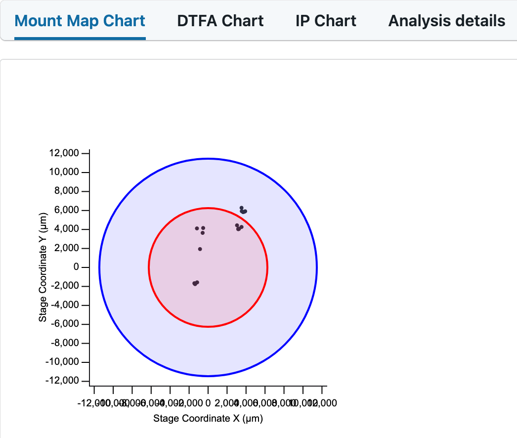
An example crossplot figure using the VX library (react + typescript/javascript) is detailed below. This is based on a crossplot for the WiscSIMS lab and you can see the code here on Github. The code for this is just the Mount Map Chart as shown below. Similar code creates the DTFA Chart and IP Chart.

Importing functions

To create your frontend figure plugin, you will need to import a number functions from some JavaScript libraries. The ones used for the example figure are in the code block below. We rely on the VX library for most of the figure creation, we use d3-array to transform the data. The library controls figure extent and what is rendered as React components.

import h from "react-hyperscript";
import React from "react";
import styled from "@emotion/styled";
import { Group } from "@vx/group";
import { scaleTime, scaleLinear } from "@vx/scale";
import { AreaClosed } from "@vx/shape";
import { LinePath } from "@vx/shape";
import { AxisLeft, AxisBottom } from "@vx/axis";
import { LinearGradient } from "@vx/gradient";
import { extent, max } from "d3-array";
import { curveMonotoneX } from "@vx/curve";
import { Point } from "@vx/point";
import { MarkerCircle } from "@vx/marker";
import { useAPIResult } from "@macrostrat/ui-components";
import { Card, Spinner } from "@blueprintjs/core";
import ReactJSON from "react-json-view";

Retrieving data

In the example figure, we get two datum for each analysis from the Sparrow database. To do this, we get the session_id from the active window with the const { session_id } = props; command. This feeds into an API call to the database to return all analyses with the current session ID. This returns more data than we need in the current iteration, so we select all data with parameter values of "X" or "Y". We return only non-null values from the stage_X and stage_Y variables with this command stage_X: stage_X?.value and the same for Y.

const { session_id } = props;
const data = useAPIResult("/analysis", { session_id }, null);
if (data == null) return h(Spinner);
const analysis_data = data.map(d => {
  const stage_X = d.data.find(d => d.parameter == "X");
  const stage_Y = d.data.find(d => d.parameter == "Y");
  return { stage_X: stage_X?.value, stage_Y: stage_Y?.value };
});

Constructing the plot area

The code below constructs the figure area. We set the constants width and height to 400 so the figure has a 1:1 aspect ratio. This is the full canvas area for the figure and contains the axis labels and plot.

Setting the margin specifies the white space above, below, right, and left of the figure.

Setting xMax and yMax finds the top right corner of the figure panel.

The xMid and yMid are particular to this figure and center the reference circles.

const width = 400;
const height = 400;

// Bounds
const margin = {
  top: 80,
  bottom: 80,
  left: 80,
  right: 80
};
const xMax = width - margin.left - margin.right;
const yMax = height - margin.top - margin.bottom;
const xMid = xMax / 2;
const yMid = yMax / 2;

Scaling the X and Y axis

The function scaleLinear from @vx/scale is used to translate the x and y scales from pixels to the units of the figure. Here we set the domain (scale in x-y units) to -12500 to 12500. The units in this case are micrometers (known from data) and this allows us to plot analysis points across a 2.5 cm round. Domains can be set automatically from the data, which is prefered if you are enabling a zoom function in your figure.

const xScale = scaleLinear({
  range: [0, xMax],
  domain: [-12500, 12500]
});

const yScale = scaleLinear({
  range: [yMax, 0],
  domain: [-12500, 12500]
});

Later in the figure creation, these functions wrap more functions. In particular these require just the X or just the Y data from farther above.

const getX = d => d.stage_X;
const getY = d => d.stage_Y;

Figure code

The figure itself is created from the following code which is almost a standalone SVG. All variables within { } are dynamically adjusted based on the data. Values within quotes (e.g. "marker-circle-1") are set once within this figure. The labels for the X and Y axis are set in AxisBottom and AxisLeft, respectively. More information on the options for adjusting axis labels can be found in the VX axis documentation.

{% hint style="warning" %} If making multiple figures with similar styling in a view within Sparrow, unique id's will need to be assigned for the MarkerCircle settings. If not, only the first figure will have points plotted! {% endhint %}

<div>
  <svg width={width} height={height}>
    <Group top={margin.top} left={margin.left}>
      <MarkerCircle id="marker-circle-1" fill="#333" size={2} />
      // This portion makes the x-y points show up on the plot.
      <LinePath
        data={culled_data}
        x={d => xScale(getX(d))}
        y={d => yScale(getY(d))}
        markerMid="url(#marker-circle-1)"
        markerEnd="url(#marker-circle-1)"
        markerStart="url(#marker-circle-1)"
      />
      <circle
        cx={xMid}
        cy={yMid}
        r={110}
        fill={"blue"}
        fill-opacity={0.1}
        stroke={"blue"}
        stroke-width={2}
      />
      <circle
        cx={xMid}
        cy={yMid}
        r={60}
        fill={"red"}
        fill-opacity={0.1}
        stroke={"red"}
        stroke-width={2}
      />
      <AxisLeft
        scale={yScale}
        top={0}
        left={0}
        label={"Stage Coordinate Y (\u03BCm)"}
        stroke={"#1b1a1e"}
        tickTextFill={"#1b1a1e"}
      />
      <AxisBottom
        scale={xScale}
        top={yMax}
        label={"Stage Coordinate X (\u03BCm)"}
        stroke={"#1b1a1e"}
        tickTextFill={"#1b1a1e"}
      />
    </Group>
  </svg>
</div>

In this figure, a central red and outer blue circle show where analyses can be precisely measured on a SIMS mount. These are set with <circle .../> from VX. The radius is in pixels and related to the pixel scale for the figure. See the code for DTFA plots for an example of dynamic scaling.

The points are added to the figure using <linepath .../> from @vx/shape but a line is not rendered because there is no information specified for the line. The specifics for this are shown again below. To render the x and y, vx expects these data to go through getX and xScale functions. We also need a unique url for the marker circles which we set above.

<LinePath
  data={culled_data}
  x={d => xScale(getX(d))}
  y={d => yScale(getY(d))}
  markerMid="url(#marker-circle-1)"
  markerEnd="url(#marker-circle-1)"
  markerStart="url(#marker-circle-1)"
/>

Enabling the plugin

Your plugin is enabled in the site-content/index.js file. To enable it, you need to add it to an existing component of Sparrow. We change the sessionDetail: output to a new series of tabs, one being the "mountMap" we detail above. We enable the MountMapChart function from the index.tsx file in the "plugins/mount-plots" folder. This adds a tab on the sessionDetail view. The example code has four tabs including "Mount Map Chart", "DTFA Chart", "IP Chart", and "Analysis details". The "Analysis details" tab is enabled by default, but must be added here if used with additional plugins.

import { Markdown } from "@macrostrat/ui-components";
import aboutText from "./about-the-lab.md";
import h from "react-hyperscript";
import { MountMapChart } from "plugins/mount-plots";
import { DtfaMountChart } from "plugins/dtfa-plot";
import { IPtimeChart } from "plugins/IP-time";
import { GLMap } from "plugins/gl-map";
import { Tab, Tabs } from "sparrow/components/tab-panel";

export default {
  siteTitle: process.env.SPARROW_LAB_NAME,
  landingText: h(Markdown, { src: aboutText }),
  sessionDetail: props => {
    const { defaultContent, ...rest } = props;
    return h(
      Tabs,
      {
        id: "sessionDetailTabs"
      },
      [
        h(
          Tab,
          { id: "mountMap", panel: h(MountMapChart, rest) },
          "Mount Map Chart"
        ),
        h(
          Tab,
          { id: "dtfaChart", panel: h(DtfaMountChart, rest) },
          "DTFA Chart"
        ),
        h(Tab, { id: "ipChart", panel: h(IPtimeChart, rest) }, "IP Chart"),
        h(
          Tab,
          { id: "analysisDetails", panel: h(defaultContent, rest) },
          "Analysis details"
        )
      ]
    );
  }
};